Stage sructured population growth with matrix models
Introduction
In most populations, individuals differ from one another in size or age. Usually these differences affect rates of survival, growth, and reproduction. For example in many plant species, small plants have a lower probability of survival than large plants. When small individuals are more abundant than large individuals, a simple average of survival probability is overly simplistic. In situations like these, we need to account for differences in transition rates due to age or stage.
In a system in which individuals are either adults, \(A\), or juveniles, \(J\). For simplictiy, we assume that individuals may only persist as adults or juveniles for one timestep.

In each timestep, the number of juveniles, \(J\), is a function of the number of adults in the prior timestep, \(A\), and their reproductive rate, \(f\).
\(J_{t+1}=A_t*f\)
Similarly, the number of adults in each timestep, \(A\), is a function of the number of juveniles in the last timestep, \(J\), that became adults at the per capita growth rate, \(g\).
\[A_{t+1}=J_t*g\]
If you remember from your algebra classes, this problem can be represented by a system of equations, because information from one equation can be used to solve the other, and vice-versa. Alternatively, we can use matrix models to summarize the dynamics of this population.
To use a matrix model, we combine the information into rows and columns that represent transitions.
\[ \left( \begin{array}{c} J \\ A \end{array} \right) = \left( \begin{array}{cc} 0 & f \\ g & 0 \end{array} \right) \]
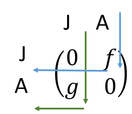
In this transition matrix, each transition is accounted for: the upper right quadrant of the matrix represents reproduction (Adults to Juveniles), the lower left represents growth (Juveniles to Adults), and the other two are set to zero, because in this simple scenario adults may not stay adults, and juveniles may not stay juveniles.

Demographic matricies are always read from the top and to the left in this way (see Figure 2), but can be expanded to include more than two stages. They are also always square, and the elements are always positive. There are two common forms of demographic matricies; leslie matricies for populations that are age-structured (individuals must progress due to age), and leftkovitch matricies where individuals may both progress and retrogress between stages. A markov matrix is different, because death rates are explictly accounted for, and we will not address those kinds of matricies here.
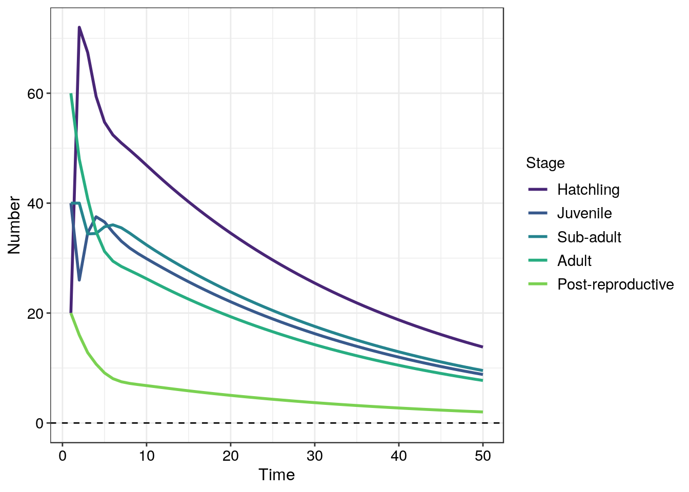
Once a demographic matrix is constructed we can simulate the dynamics of the population in discrete time, or we can use the matrix to calculate asymptotic (the long-term) behavior. In a deterministic framework, both approaches should ultimately result in the same answer. The example above is relatively simplified, in reality there are few species that just have a juvenile and adult stage. In today’s example you will work with a matrix consisting of five stages with four variables for each stage of the population; its initial size \(N_0\), birth rate \(b\), growth rate \(g\), and probability that an individual will remain at a particular stage rate \(r\).
Researchers use these stage structured models in many ways. A popular application is to identify which stages of the population are more sensitive than others. The purpose here is to identify which apsects of the population respond best (or worst) to various conservation efforts. Should we base our conservation on promoting high egg laying rates or should we focus on ensuring that hatchlings make it into the sea safely to grow up to become juveniles? Those are just some of the questions that can be answered in part by what are caled sensitivity and elasticity analyses.
Remember to think carefully about the values you are inputting. You have three parameters, probability of successfully reproducing, probability of remaining, and the probability of growing. If the sum of of these latter two probabilities is greater than 1 then your model will result in an incorrect output - please remember that. You cannot have more individuals at the end of an age class (from the same initial cohort) than what you started with at the beginning of a given time period. A good way to thing about how you manipulate these probabilities is to decide first how many individuals will grow - let’s say 0.5 or 50%. That leaves us with 50% to assign the number of individuals that will remainin in an age class. Let’s make this value .02 or 20%. Then that leaves 0.3 unaccounted for - those are the individuals which have died.
Download the staged structured growth app here and complete the prac worksheet questions.
Worksheet questions (32)
Stage structured population growth
Question 1
Do not change any of the parameters of the Shiny App before attempting this question – if you have then restart or reload the app. Write out a matrix equation that illustrates the population composition at time t+1 based on the population at time t and the transition matrix (4)
Question 2
Sensitivity and elasticity are two terms used to describe how important each transition arrow in the life cycle diagram is in determining \(\lambda\). Sensitivity is an arrow’s (or transition’s) direct contribution to \(\lambda\) - high sensitivity means that small changes in a transition pararmeter will have great effects on \(\lambda\) where \(\lambda\) is the populations growth rate once it is stabilised. This can be calculated manually by modelling the population for many years and calculating lambda once no change in the proportions of the different classes is occurring. Alternatively, \(\lambda\) can be calculated as the main or dominant eigenvalue of the Leslie (\(l\)) matrix. The contribution of each element in the Leslie matrix (\(l_{ij}\)) to \(\lambda\) can then be calculated as
\[ \frac{\partial \lambda_{1}}{\partial l_{ij}} = \frac{(w_{1}){i}(v_{1})_{j}}{\bar{w}_{1}^{T} \bar{v}_{1}} \] where \(w_{1}\) and \(v_{1}\) are left and right eigenvectors of the dominant eigenvalue (which is \(\lambda\)). For interest, This video provides some further explanation on these terms.
Once we have this sensitivity matrix wer can calculate a standardised measure of sensitivity - this is called elasticity. In this case sensitivity is weighted by \(\frac{l_{ij}}{\lambda}\) - the corresponding Leslie matrix value divided by the population’s net growth rate.
Manipulate the parameters of the Shiny App one by one and explain how the class’ elasticty generally changes in response to your parameter manipulations. Discuss, given the starting model parameters, which class is the most and which is the least important to ensuring the population’s survival (10)
Question 3
Under what conditions will the population experience 1. a “baby-boom” (3) 2 become extinct as a result of an “aging population” (3)
Question 4
A population of grasshoppers in the KwaZulu-Natal south coast has initial population sizes of
\[ \left[ \begin{array}{c} Nymphs \\ Sub-adults \\ Adults \end{array} \right] = \left[ \begin{array}{cc} 10 \\ 13 \\ 3 \end{array} \right] \] And the population’s probabilities of transitioning between states is described as:

- Construct the Leslie matrix which describes this transition matrix (4)
- Calculate the number of individuals for each stage for the next two time periods (8)
Coding questions
The graph produced using the Shiny App is interesting but there are several other ways in which these structured population models can be presented. By altering the working code below produce plots which present
- the stage population sizes and add in the total population size (4)
- present your previous plot2 on the log scale for population size (3)
- present the stage sizes as a proportion of the total population and do not plot total population size (4)
list.of.packages <- c("dplyr", "tibble", "tidyr", "ggplot2", "viridis")

#checking missing packages from list
new.packages <- list.of.packages[!(list.of.packages %in% installed.packages()[,"Package"])]

#install missing ones
if(length(new.packages)) install.packages(new.packages, dependencies = TRUE)


nSteps <- 50 # number of time steps

popvec <- matrix(c(20, 40, 40, 60, 20),
                 nrow = 5,
                 ncol = 1) #initial population size vector
tmat <- matrix(c(0.1, 0.1, 0.6, 0.7, 0,
                 0.3, 0.5, 0,   0,   0,
                 0,   0.4, 0.6, 0,   0,
                 0,   0,   0.3, 0.6, 0,
                 0,   0,   0,   0.2, 0.2),
               nrow = 5, ncol = 5,
               byrow = T) # Leslie matrix

# make a wide matrix where each column is a time step and each row is a stage class
# vec is the population size vector at time t-1
# vec is then added to the right hand side of popvec
for (i in 2:nSteps) {
  vec <- matrix(popvec[,i - 1],
                ncol = 1,
                nrow = 5,
                byrow = T)
  popvec <- cbind(popvec, tmat %*% vec)
}

colnames(popvec) <- seq(from = 1, to = nSteps, by = 1) # makes the column names of popvec equal to the time step the column represents
popvec <- as.data.frame(popvec) # convert popvec to a dataframe
rownames(popvec) <- c("Hatchling",
                      "Juvenile",
                      "Sub-adult",
                      "Adult",
                      "Post-reproductive") # make the rownames represent the stage classes
popvec <- popvec %>%
  rownames_to_column(var = "Stage") %>% # covert these rownames to the first column
  gather(key = "var",
         value = "Number",
         -Stage) %>% # gather in all the population sizes for each class resulting in one column for class (Stage), one column for number of individuals in that class (Number) and the time step (currently var) but do not include Stage in this - that way it will preseve those data for each combination
  select(Stage, Number, "Time" = var) # select those columns in a particular order and rename var to Time

popvec$Time <- as.numeric(popvec$Time) # convert time from character to numeric
popvec <- popvec %>%
  arrange(Stage, Time) # arrange the dataframe by Time within Stage

popvec$Stage <- factor(popvec$Stage, levels = c("Hatchling",
                                                "Juvenile",
                                                "Sub-adult",
                                                "Adult",
                                                "Post-reproductive")) # assing levels to the stage classes which controls their ordering in the plot output

ggplot(dat = popvec) +
  geom_line(mapping = aes(x = Time, y = Number, colour = Stage), size = 1) +
  geom_hline(yintercept = 0, linetype = 2) + # adds the (dotted) horizontal line intercepting y at 0
  theme_bw() + # choose the black and white theme
  theme(axis.title = element_text(colour = "black",
                                  size = 12), # change axis title text colour to black and size to 12
        axis.text = element_text(colour = "black",
                                 size = 11), # change axis number text colour to black and size to 11
        legend.text = element_text(colour = "black",
                                 size = 11)) + # change legend label text colour to black and size to 11
  scale_colour_viridis(discrete = TRUE, begin = 0.1, end = 0.8) # use the viridis colour palette for the different stages
Application questions (35)
Question 1
Discuss the differences between age and stage structured population growth matrix models. Give examples of four species that would be suitably modelled by both of these types of matrix models (12)
Question 2
In our examples we have assumed that individuals of the population can either remain in a given stage or progress on to the next stage. There are in fact scenarios where individuals may regress or go back a stage. Give a brief overview of how this kind of growth differs from the general stage structured growth and give four examples of what kinds of populations this might exhibit this kind of growth and explain in brief the mechanism the population uses to grow in that way. Also provide an example transition matrix to illustrate how a population of this nature might be modelled using a Leslie matrix (10)
Question 3
Hunting or commercial harvesting can drastically affect population sustainability and viability and so the harvesting of populations (particularly the more sensititve populations) is often strongly legislated. Discuss how these kinds of population growth models and analyses can be incorporated into legislating harvesting of natural populations. Make reference to both scientific publications and government policies (13)